Habitat Suitability for Bison bison in The United States
How Environmental Factors Affect Range
Jessica Wood

Bison bison
Introduction
Species ranges are restricted based on the ecological features they are suited to inhabit. This constraint can cause a species’ range to exist as highly fragmented populations or be relatively ubiquitous over a large area based on the location of these features. Bison populations are subject to this range restriction, preferring habitats with a large amount of open area, drier climates and mid-range elevations where grasses grow well (Lott,2017). Due to these assumptions it is expected that bison would be found in areas that meet all or most of these standards. In order to examine how habitats are able to affect bison populations and their locations, species observations can be used to determine which habitat types are most suitable for bison and where they are located (Palma,1999). From this analysis a map of locations that are suitable for bison will be created based on a selected model. From this map it is expected that highly suitable points will be found within Yellowstone National Park, as it is the only location within the United States with a wild bison herd (Gates,2008). Additionally, it is expected that locations with mid- to high-elevations, mid-range climates and low forest cover will be most suitable for the species.
Materials and methods
Install and load required packages:
library(spocc)
library(spThin)
library(dismo)
library(rgeos)
library(ENMeval)
library(raster)
library(dplyr)
library(knitr)
library(wallace)
library(leaflet)
library(widgetframe)
library(DT)
opts_chunk$set(cache=T)
The wallace package also requires functions that are not included with the package. The function system.file will find them and source will load it:
source(system.file('shiny/funcs', 'functions.R', package='wallace'))Obtating Occurence Data
Occurance data will be downloaded from the gbif database (GBIF,2017). The data retrieval tool within the wallace package limited this download to 3000 records and therefore this dataset does not contain all occurrence data points.
results <- spocc::occ(query = "Bison bison", from = "gbif", limit = 3000, has_coords = TRUE)
results.data <- results[["gbif"]]$data[[formatSpName("Bison bison")]]
occs <- remDups(results.data)
Rows where coordinates are duplicates must be removed. Latitudes and longitudes must also be checked to be sure they are numeric.
occs$latitude <- as.numeric(occs$latitude)
occs$longitude <- as.numeric(occs$longitude)
Collected records can all be labeled with unique names.
occs$origID <- row.names(occs)The data then needed to be filtered to only include observations located within the continental United States In total 2957 observations were selected. These observations were then edited to only include 625 observations in order to minimize processing time.
a=filter(occs,longitude<0)
occs=filter(a,latitude<50)
A data table containing a summary of these points as well as a map created to show their location can be found in Table 1 and Figure 1.
Environmental Data
Data was collected from the WorldClim (Fick,2017) database using a resolution of 2.5 arc minutes.
preds <- raster::getData(name = "worldclim", var = "bio", res = 2.5, lat = , lon = )
locs.vals <- raster::extract(preds[[1]], occs[, c('longitude', 'latitude')])
Occurance points that were not associated with any environmental data were removed.
occsenv <- occs[!is.na(locs.vals), ] A bounding box was created to surround all points included in the dataset. This will also exlude areas where no observations are found. Additionally, no buffer was used to avoid the inclusion of Canada and Mexico in the analysis.
xmin <- min(occsenv$longitude) - (0 + res(preds)[1])
xmax <- max(occsenv$longitude) + (0 + res(preds)[1])
ymin <- min(occsenv$latitude) - (0 + res(preds)[1])
ymax <- max(occsenv$latitude) + (0 + res(preds)[1])
bb <- matrix(c(xmin, xmin, xmax, xmax, xmin, ymin, ymax, ymax, ymin, ymin), ncol=2)
backgExt <- sp::SpatialPolygons(list(sp::Polygons(list(sp::Polygon(bb)), 1)))
A study extent was generated that included only the enviromental variables in the bouding box using a mask. A random sample was also taken from the generated study extent. 10,000 background values were used, however, a larger number would decrease variablity in the results.
predsBackgCrop <- raster::crop(preds, backgExt)
predsBackgMsk <- raster::mask(predsBackgCrop, backgExt)
occs.locs <- occsenv[,2:3]
bg.coords <- dismo::randomPoints(predsBackgMsk, 10000)  # generate 10,000 background points
bg.coords <- as.data.frame(bg.coords)  # get the matrix output into a data.frame
Partition Occurance Data
The model being constructed needs to be validated through testing. This can be done by partitioning the observation data-points into multiple sets. Here, the data was broken up into four sets of points which will then be placed in the model three at a time to check for accuracy.
group.data <- ENMeval::get.block(occ=occs.locs, bg.coords=bg.coords)modParams <- list(occ.pts=occs.locs, bg.pts=bg.coords, occ.grp=group.data[[1]], bg.grp=group.data[[2]])Choose and Evaluate Niche Model
The BIOCLIM model was used to create a distribution model for this species.The goal of this model is to find a rule that applies to all or most of the areas of a similar climate that contain species observations.
e <- BioClim_eval(modParams$occ.pts, modParams$bg.pts, modParams$occ.grp, modParams$bg.grp, predsBackgMsk)
evalTbl <- e$results
evalMods <- e$models
names(e$predictions) <- "Classic_BIOCLIM"
evalPreds <- e$predictions
occVals <- raster::extract(e$predictions, modParams$occ.pts)  # get predicted values for occ grid cells
mtps <- min(occVals)  # apply minimum training presence threshold
# Define 10% training presence threshold
if (length(occVals) < 10) {  # if less than 10 occ values, find 90% of total and round down
  n90 <- floor(length(occVals) * 0.9)
} else {  # if greater than or equal to 10 occ values, round up
  n90 <- ceiling(length(occVals) * 0.9)
}
p10s <- rev(sort(occVals))[n90]  # apply 10% training presence threshold
Project Model
projCoords <- data.frame(x = c(-123.7456, -94.3022, -80.3276, -70.3081, -67.3198, -78.7456, -81.1187, -88.9409, -98.0815, -104.6733, -118.5601, -124.7124), y = c(49.153, 49.2678, 42.033, 47.2792, 45.4601, 33.7974, 26.116, 30.4487, 26.116, 29.5352, 32.6949, 42.2285))
projPoly <- sp::SpatialPolygons(list(sp::Polygons(list(sp::Polygon(projCoords)), ID=1)))

# Selected model from the evalMods list
modSel <- evalMods[[1]]
Map Projected Model
predsProj <- raster::crop(preds, projPoly)
predsMsk <- raster::mask(predsProj, projPoly)

newExtProj <- dismo::predict(modSel, predsMsk)
plot(newExtProj)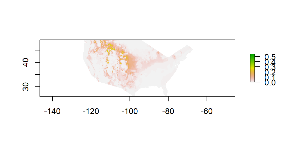
Habitat Distribution of Bison bison Within The United Sates
Extend to New Time
This model can then be extended to a new time frame, such as 2070. This can be done using General Circulation Models and Concentration Pathways.
predsFuture <- raster::getData("CMIP5", var = "bio", res = 2.5, rcp = 85, model = "HG", year = 70)

predsProj <- raster::crop(predsFuture, projPoly)
predsMsk <- raster::mask(predsProj, projPoly)

# rename future climate variable names
names(predsMsk) <- names(preds)
futureProj <- dismo::predict(modSel, predsMsk)
plot(futureProj)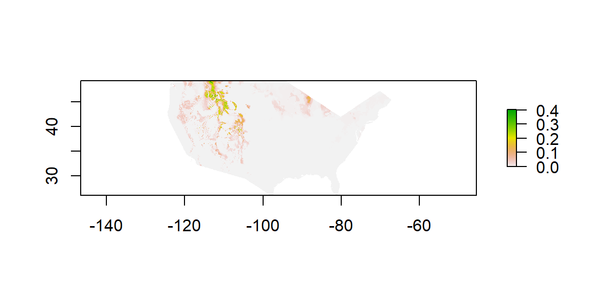
Map of Bison Habitat in 2070
Results
Table 1: Bison Observations
datatable(occs, options = list(pageLength = 5))Bison Observations in the United States
Figure 1: Observation Map
leaflet(occs) %>% addProviderTiles(providers$OpenStreetMap) %>% addMarkers(
  clusterOptions = markerClusterOptions(maxClusterRadius=20)
) %>% frameWidget(height =500)
## Assuming 'longitude' and 'latitude' are longitude and latitude, respectivelyMap of Observation Data Within The United Sates
This map shows the raw occurrence data that was found to be within the United States limits.This map only includes 625 data points from a total of almost 3000 possible in order to accelerate processing time.It can be seen that while bison observations are widespread across the United States, there is a preference of the species towards the western portion of the country.
Figure 2: Modeling Results
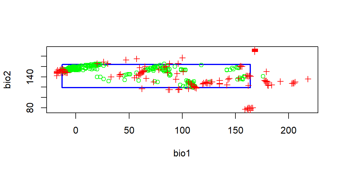
Results of Modeling Analysis for Bio 1 and 2
Bioclim compares the values of environmental factors at locations with known occurrence data in order to find areas with similar climates. In this example Bio1 is the annual mean temperature of the area, while Bio2 is the locations mean diurnal range (average of daily maximum minus daily minimum temperature per month). Green points show the occurrence locations and red points are absence data. This model then creates an envelope where occurrence points are found in each combination of climate data in order to make assumptions regarding the preferred habitat of the species.
Table 2: Model Selection
| Mean | Variance | Bin 1 | Bin 2 | Bin 3 | Bin 4 | |
|---|---|---|---|---|---|---|
| AUC.DIFF | 0.280 | 0.112 | 0.498 | 0.420 | 0.007 | 0.195 |
| AUC.TEST | 0.608 | 0.090 | 0.397 | 0.507 | 0.854 | 0.675 |
| OR10 | 0.553 | 0.310 | 0.810 | 0.829 | 0.033 | 0.539 |
| ORmin | 0.352 | 0.193 | 0.673 | 0.507 | 0.020 | 0.211 |
Table 1 and Figure 2 are both results of the modeling analysis. Area under the curve (AUC) is the ability of a model to discriminate between presence and absence data, therefore, it should be high in a suitable model. The omission rate (OR) of a model indicates how often observations fall outside the prediction area. Both minimum traning and 10 percent training both apply to the omission rate, with 10 percent being a more strict analysis (Jamie,2017).Due to the resulting output, the best combination of AUC and OR is Bin 1, with a mid -range AUC but a lower OR for both minimum and 10 percent training and will be used in the model.
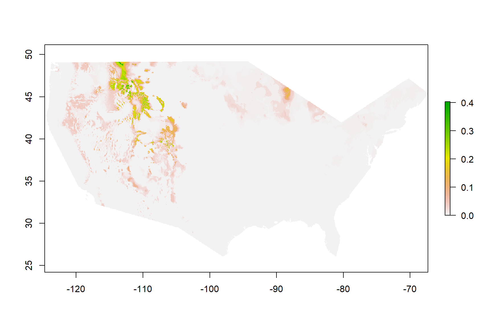
Figure 3: Current Habitat
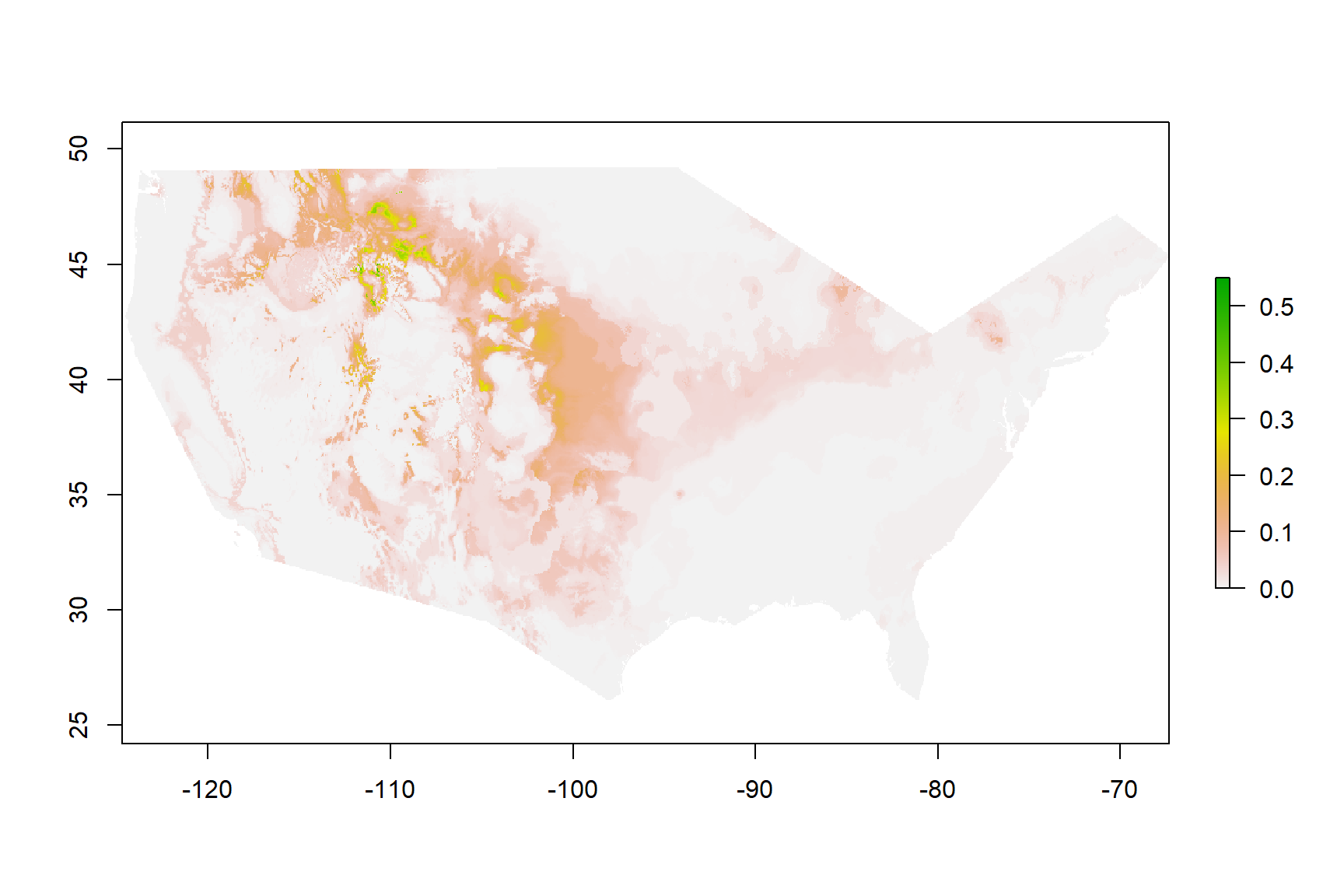
Habitat Distribution of Bison bison Within The United Sates
Figure 3 are the results of habitat modeling for Bison bison in the United States. A high value, labeled in green, would apply to any area that is suitable bison habitat. A low value or a value of 0 indicates a location where it would be difficult for bison to exist in currently. It can be noted that higher values can be seen in the North Western United States. This approximation makes sense due to the knowledge that currently bison herds live in this area near Yellowstone National Park.
Figure 4: 2070 Habitat
Map of Bison Habitat in 2070
Figure 4 maps the distribution of bison habitat that could occur in 2070 if current climate trends continue. This habitat appears to shift towards the northwest. Additionally, areas of high suitability become more concentrated and areas of low suitability turn into areas of 0.0. This map is only based on a single climate model and concentration pathway combination.
Conclusions
625 bison observations within the United States were analyzed in order to determine where suitable habitat for the species is located. After selecting an appropriate model, the resulting map showed that a majority of the highly suitable habitat within the country can be found in the Northwest. While there is a very limited number of highly suitable locations, areas of lower suitability are widespread across the US. This data was then projected into the future using climate models and carbon concentration pathways. This resulted in very few highly suitable areas that continue to move northwest, as well as the shrinking of area of lower suitability. This analysis could be redone using different combinations of climate and carbon projections in order to determine the broader implications of climate change on the species Bison bison, as well as aid in the preservation of the species that is currently environmentally confined.
References
Fick, S.E. and R.J. Hijmans, 2017. Worldclim 2: New 1-km spatial resolution climate surfaces for global land areas. International Journal of Climatology.
Gates, C., & Aune, K. (2008). Bison bison. Retrieved November 1, 2017, from http://dx.doi.org/10.2305/IUCN.UK.2008.RLTS.T2815A9485062.en.
GBIF.org (10th October 2017) GBIF Occurrence Download
Jamie M. Kass, Bruno Vilela, Matthew E. Aiello-Lammens, Robert Muscarella and Robert P. Anderson (2017). wallace: A Modular Platform for Reproducible Modeling of Species Niches and Distributions. R package version 0.6.4. https://CRAN.R-project.org/package=wallace
Lott, D. F. (n.d.). American Bison: A Natural History. Retrieved from https://books.google.com/books?hl=en&lr=&id=bHQlDQAAQBAJ&oi=fnd&pg=PR9&dq=american+bison+habitat&ots=GEnYiHphVa&sig=uevTRwdpaDtYGrK8ZUzF6zjwZhI#v=onepage&q=american bison habitat&f=false
Palma, L., Beja, P., & Rodrigues, M. (1999). The use of sighting data to analyse Iberian lynx habitat and distribution. Journal of Applied Ecology, 36(5), 812–824. http://doi.org/10.1046/j.1365-2664.1999.00436.x